Hands-on tutorial to get started with deep learning using Sci-kit learn

In this post, I will introduce you to a machine learning method called Supervised Learning. And I will show you how to build a kNN Classifier model using Sci-kit learn. This will be a hands-on walkthrough where we will be able to learn while practicing our knowledge. As our classifier model, we will use the k-NN model, which will be covered more in the introduction section. After reading this tutorial, you will have a better understanding of deep learning and how supervised learning models work. If you are ready, let’s get started!

Table of Contents:

• Supervised Learning
• Libraries
• The Digits Data
• k-NN Classifier Model
• Overfitting and Underfitting
• Conclusion

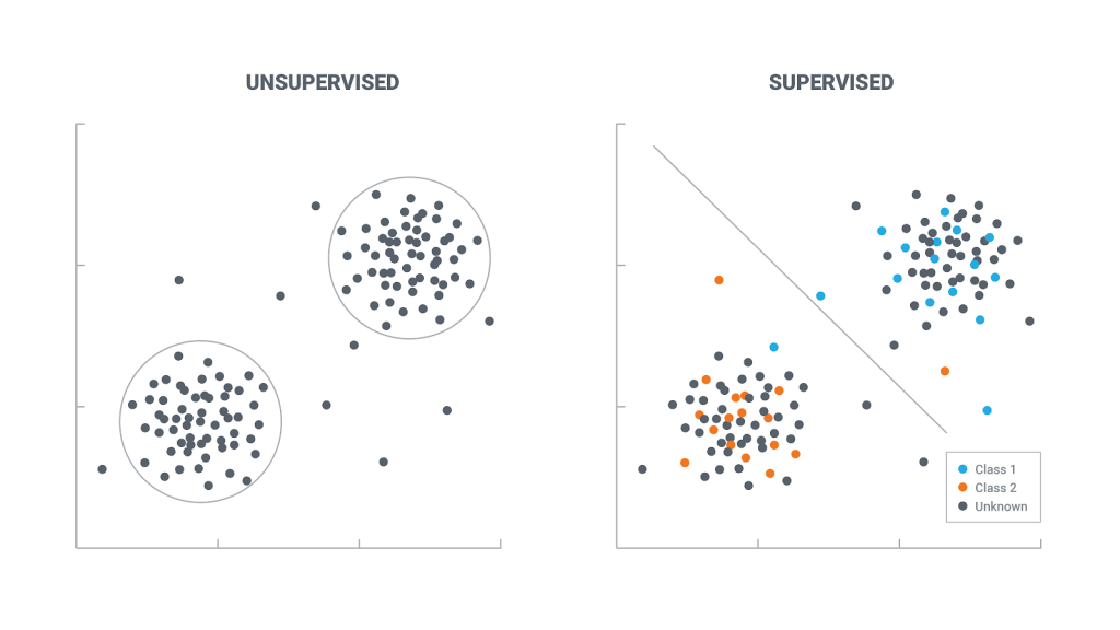
Supervised Learning

Deep learning is the science of giving computers the ability to learn to make conclusions from data without being explicitly programmed. Such as learning to predict whether an email is a spam or not. Another great example can be clustering flower species into different categories by looking at their pictures.

In supervised learning, the data is divided into two parts: features and target variables.
The mission is to predict the target variable by looking at the features variables.
Supervised learning can be used in two different models: Classification and Regression.
Classification models can be used when the target variables are categorical datasets. Regression models are being used when the target variables are continuous values.

Libraries

In this step, we will install the libraries that we will need for this tutorial. As mentioned in the introduction, the main deep learning library we will use is called Sci-kit learn. Other than that, we will install two simple libraries, and they are NumPy and Matplotlib. Installation of the libraries is straightforward using PIP, which is a python package manager. Let’s go to our terminal window and write the following lines to begin the installation process:

pip install scikit-learn

Now let’s install the other two libraries in one line:

pip install NumPy matplotlib

Import libraries

Perfect! Now let’s import them to our program so that we can use them. I will be using Jupyter Notebook in this tutorial. So, I created a new notebook and imported the following modules of libraries. You will understand each of them as we begin using them in the next steps. 

from sklearn import datasets
from sklearn.neighbors import KNeighborsClassifier 
from sklearn.model_selection import train_test_split 
import matplotlib.pyplot as plt
import numpy as np

The Digits Data

For this exercise, we will use the digits data. It is also known as the MNIST. This is a famous data to get started with building a supervised learning model. And the good thing about this data is we don’t have to download anything; it comes with the sklearn module that we installed earlier. Here is how we load the dataset:

digits = datasets.load_digits()

Now, let’s try to have some understanding of the dataset running a couple of lines.

print(digits.keys)

#A Bunch is a Python dictionary that provides attribute-style access. Bunch acts like an object and a dictionary.

print(digits.DESCR)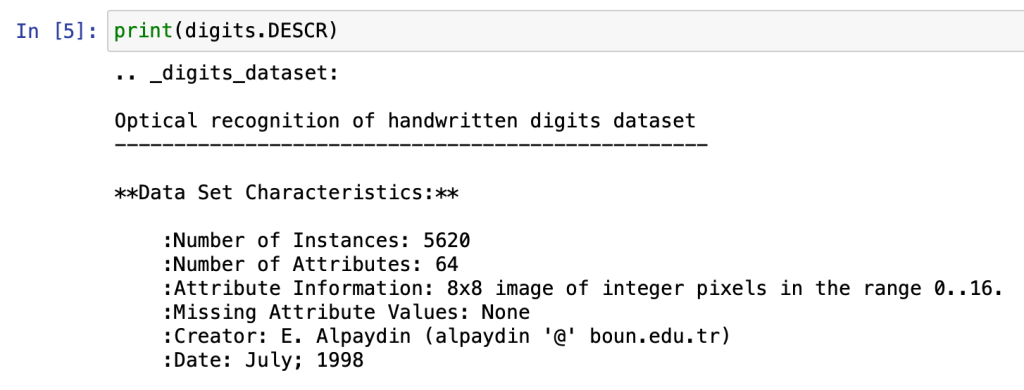

print(digits.data.shape)

plt.imshow(digits.images[1010], cmap=plt.cm.gray_r, interpolation='nearest')

plt.show()

k-NN Classifier Model

“The k-nearest neighbor algorithm (k-NN) is a non-parametric method proposed by Thomas Cover used for classification and regression. In both cases, the input consists of the k closest training examples in the feature space. The output depends on whether k-NN is used for classification or regression.”

Reference: https://en.wikipedia.org/wiki/K-nearest_neighbors_algorithm

We have already imported the k-NN Classifier module in the Libraries step. So, all we have to do is use it on our dataset. This step is a nice exercise of using a ready sklearn module on a project. Since we are doing supervised learning, the dataset has to be labeled. This means when training the data, we are also teaching the outcomes. 

Data and target attributes

The digit data has two attributes, which are data and target. We will start by assigning these parts to new variables. Let’s call our features X and the labels y. We can do this easily using attributes.

X = digits.data
y = digits.target

Train_and_split

Next, we will use the train_and_split method to split our data part. Instead of training the whole data, it’s a better practice to split it into training and testing data to review our models’ accuracy. This will make more sense in the next step, where we will see how to improve the predictions using some methods. 

Here is how to split the data:

X_train, X_test, y_train, y_test = train_test_split(X, y, test_size = 0.2, random_state=42, stratify=y)

Neighbors

knn = KNeighborsClassifier(n_neighbors = 7)

Fitting the model

knn.fit(X_train, y_train)

Accuracy

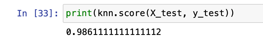
print(knn.score(X_test, y_test))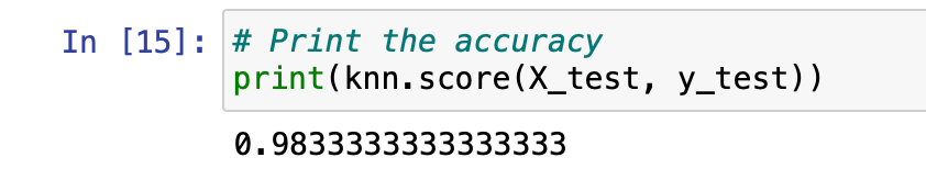

Let me show you how this score is calculated.
First, we are making a prediction using the knn model on the X_test features.

y_pred = knn.predict(X_test)

and then comparing it with the actual labels, which is the y_test.
Here is how the accuracy is calcuated:

number_of_equal_elements = np.sum(y_pred==y_test)
number_of_equal_elements/y_pred.shape[0]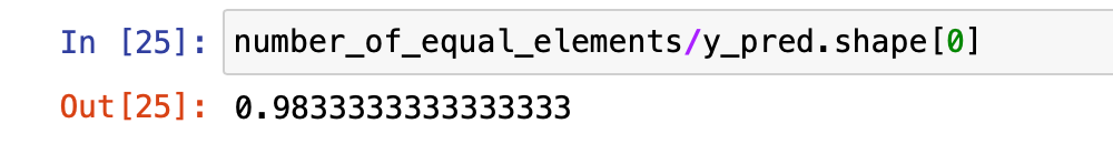

Overfitting and Underfitting

Here is nice explanation of overfitting a underfitting of the mode by Amazon machine learning course documentation:

The model is underfitting the training data when the model performs poorly on the training data. This is because the model is unable to capture the relationship between the input examples (features) and the target values (labels). The model is overfitting your training data when you see that the model performs well on the training data but does not perform well on the evaluation data. This is because the model is memorizing the data it has seen and is unable to generalize to unseen examples.

https://docs.aws.amazon.com/machine-learning/latest/dg/model-fit-underfitting-vs-overfitting.html

Now, let’s write a function that will help us see how our data performs in different neighbor values. This function will also help us analyze how the model performs the best, which means more accurate predictions.

neighbors = np.arange(1, 9)
train_accuracy = np.empty(len(neighbors))
test_accuracy = np.empty(len(neighbors))

for i, k in enumerate(neighbors):
  knn = KNeighborsClassifier(n_neighbors = k)
  #Fit the classifier to the training data
  knn.fit(X_train, y_train)
  #Compute accuracy on the training set
  train_accuracy[i] = knn.score(X_train, y_train)
  #Compute accuracy on the testing set
  test_accuracy[i] = knn.score(X_test, y_test)

Now, let’s plot the results:

plt.title('k-NN: Varying Number of Neighbors')
plt.plot(neighbors, test_accuracy, label = 'Testing Accuracy')
plt.plot(neighbors, train_accuracy, label = 'Training Accuracy')
plt.legend()
plt.xlabel('# of Neighbors')
plt.ylabel('Accuracy')
plt.show()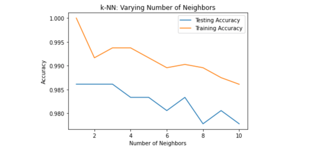

This plot proves that more neighbors don’t always mean better performance. It mostly depends on the model and the data, of course. In our case, as we can see, testing accuracy is highest for 1-3 neighbors. Earlier, we trained our knn model with 7 neighbors, and the accuracy score we got was 0.983. So, now we know that our model performs better with 2 neighbors. Let’s retrain our model and see how our predictions will change.

knn = KNeighborsClassifier(n_neighbors = 2)
knn.fit(X_train, y_train)
print(knn.score(X_test, y_test))

Conclusion

Perfect! You have created a supervised learning classifier using the sci-kit learn module. We also learned how to check how our classifier model performs. We also learned about overfitting and underfitting, which allows us to improve the predictions. Deep learning is so fun and amazing. I will share more deep learning articles. Stay tuned!

I am so glad if you learned something new today. Feel free to contact me if you have any questions while implementing the code. 😊

Follow my blog and youtube channel to stay inspired. Thank you,